

The Kalman Filter [1] originally by R. E. Kalman, is an algorithm used in control systems and signal processing to estimate the state of a system over time from a series of noisy measurements. The filter works in two steps: prediction and update. The prediction step uses the current state and a mathematical model of the system to predict the next state which includes uncertainty via the error covariance. When a new input is received, the filter performs the update step by updating the predicted state using the new input. The predicted state and new input are combined in a way that minimizes uncertainty.
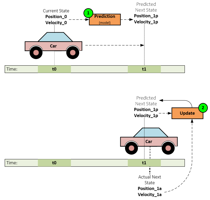
For example, imagine you want to track the position and speed of a moving object, like a car, over time. The car’s state at any time can be described by its position and speed. Sensors provide the measurements of the car’s position and speed, but these measurements are noisy and not perfectly accurate. Based on the current position and speed of the car and the mathematical model of the car’s motion, the filter predicts the car’s state at the next ‘future’ time-step which also contains some uncertainty. When a new measurement is received of the car’s new actual position and velocity, the filter updates the predicted state using the latest information by combining the predicted state and the new measurement in a way that minimizes uncertainty.
In its original form, the Kalman Filter (KF) works well on linear systems because the filter primarily relies on Linear Algebra operations for the prediction and update steps. To learn more about how the original KF works, see the great tutorials provided by Becker [2] and e-book by Labbe [3].
An alteration to the original KF called the Unscented Kalman Filter (UKF) by Wan et al. [4] has been successfully applied to non-linear systems such as those found in financial time-series data streams. The e-book by Labbe [3] has a great discussion on the UKF and how it is derived.
Using the Unscented Kalman Filter on Stock Price Data
This post demonstrates how to use the UKF to filter and smooth stock market data using the UKF implementation provided by the open-source GitHub project called filterpy by Labbe [5].
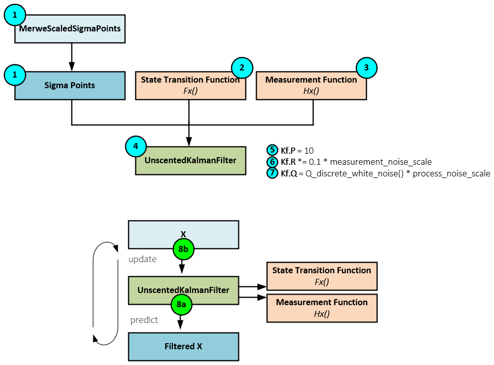
Using the UKF involves the following steps:
-
- Generate the initial signal points using the MerweScaledSigmaPoints function which implements the Merwe algorithm discussed in [6]. Note, the defaults work well in most applications.
- Define the state transition function fx used to predict the next state by transforming the current state with the sigma points from the current time step to the predicted state for the next time step.
- Define the measurement function hx used to update the sigma points from state space to the measurement space helping estimate the predicted measurement mean and covariance, which are used to update the new state estimate and its covariance.
- Create the UnscentedKalmanFilter (UKF) passing to it the sigma points, and the fx and hx functions.
- Set the P covariance matrix representing the covariance of the state estimate.
- Scale the R measurement noise covariance matrix. Increasing the scale makes the filtered values smoother.
- Scale the Q process noise covariance matrix. Decreasing the process noise makes the filtered values smoother.
- And finally, filter the data by predicting the next value then updating the filter with the next actual value. Continue the predict/update process through each point of the data being filtered.
Sigma Points
The sigma points are generated using the MerweScaledSigmaPoints as shown below. In general, the default settings work well for most applications. For more details on how these points are created see [6] and [3]. The set of sigma points provides a deterministic sampling of the mean and covariance which works surprisingly well for most data sets to propagate the distribution of the state through the nonlinear system and measurement functions.
points = MerweScaledSigmaPoints(2, alpha=0.1, beta=2., kappa=0)
Plotting the sigma points with the mean state and covariance matrix blow…
# Example state mean and covariance
x = np.array([2, 2])  # mean state
P = np.array([[1, 0.5], [0.5, 1]])  # covariance matrix
…produces the following plot.
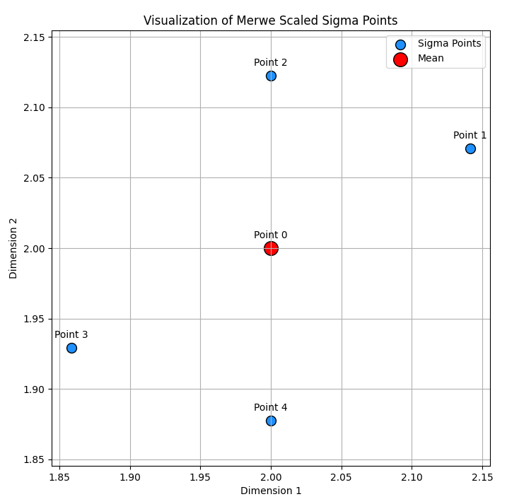
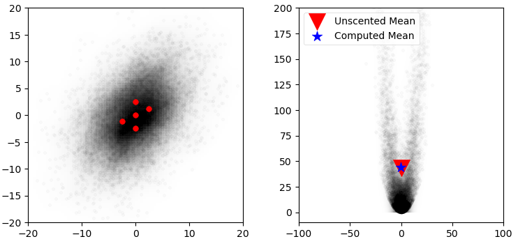
Labbe [3] demonstrates that these 5 points generated using the Merwe algorithm [6] can compute the mean with very good accuracy thus providing a large optimization over methods used by the Extended Kalman Filter (EKF).
State Transition Fx Function
The state transition fx function defines how the system evolves over time by calculating the predicted next state given the current state and the interval of time transpiring between each state.
# Define the state transition function
def fx(x, dt):
    F = np.array([[1, dt],
                  [0, 1]])
    x1 = np.dot(F, x)
    return x1
In our stock price example, we use the current price (position) and add the price change (velocity) between time steps where x = (price, velocity) and dt = the time increment.
Measurement Hx Function
For the measurement function we just return the stock price at the current time step.
# Define the measurement function
def hx(x):
    return np.array([x[0]])
For this simple model, we ignore the price velocity in the measurement function and only return the current price as the position.
Unscented Kalman Filter Initialization
When creating the UKF, the points created by the MerweScaledSigmaPoints function, the fx state transition function, and the hx measurement function are all passed to the UKF class. In addition, the initial x state is set to 0 and the P covariance matrix, R measurement noise covariance matrix, and Q process noise covariance matrix are all initialized.
# Define the initial state
dt = 1.0  # Time step (1 day)
x_initial = np.array([prices[0], 0])  # Initial state [price, velocity]
measurement_noise = 10  # increase to make the curve smoother
process_noise = 0.01      # reduce to make the curve smoother
display_uncertainty = True

# Define the process and measurement noise
points = MerweScaledSigmaPoints(2, alpha=0.1, beta=2., kappa=0)
kf = UKF(dim_x=2, dim_z=1, fx=fx, hx=hx, dt=dt, points=points)
kf.x = x_initial
kf.P *= 10  # Initial covariance
kf.R = 0.1 * measurement_noise  # Measurement noise
kf.Q = Q_discrete_white_noise(dim=2, dt=dt, var=0.1) * process_noise  # Process noise
The scaling of the R and Q covariance matrices impacts the smoothness of the filter output. To create a smoother curve, increase the measurement noise to 10 and decrease the process noise to 0.01. See later in the post for other examples to get a feel for how these settings work.
Filtering the Data
Filtering the data involves iteratively predicting the next point, then updating with the next actual point. Each predicted point makes up the newly filtered output data.
# Run the filter on historical data
filtered_prices = []
for price in prices:
    kf.predict()
    kf.update(np.array([price]))
    filtered_prices.append(kf.x[0])
Once completed, the filtered_prices array will contain the newly filtered data.
Results
In this section, we analyze the price data for ‘AAPL’ for the past year (ending on 6/30/2024).
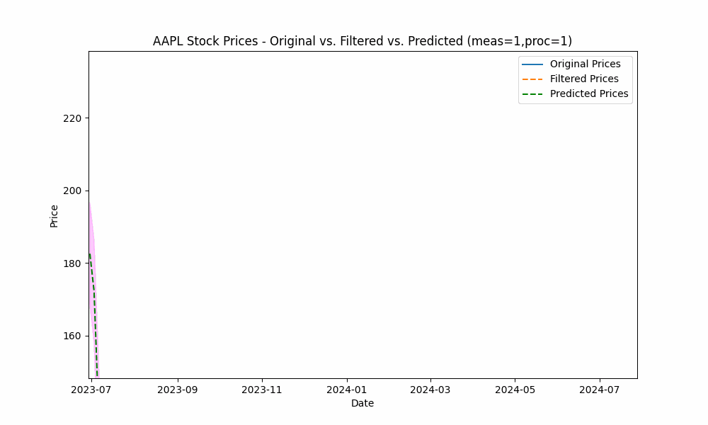
In our first run, we set the measurement_noise_scale = 1 and the process_noise_scale = 1 which produces a filter that closely tracks the price. The green dotted line shows the 10-point future prediction at each point with the model confidence levels shown in pink.
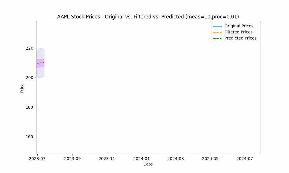
To smooth out the curve, let us increase the measurement noise scale to 10 and decrease the process noise scale to 0.01.
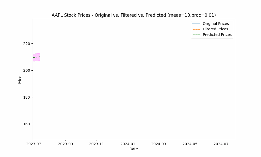
With these changes, the predicted line is now smoother, yet tracks the price movement well.
Increasing the measurement noise adds uncertainty to the measurements thus causing the filter to place more trust in the process model. In the same way, decreasing the process noise increases the filter’s trust in the process model giving it more impact on the filtered results.
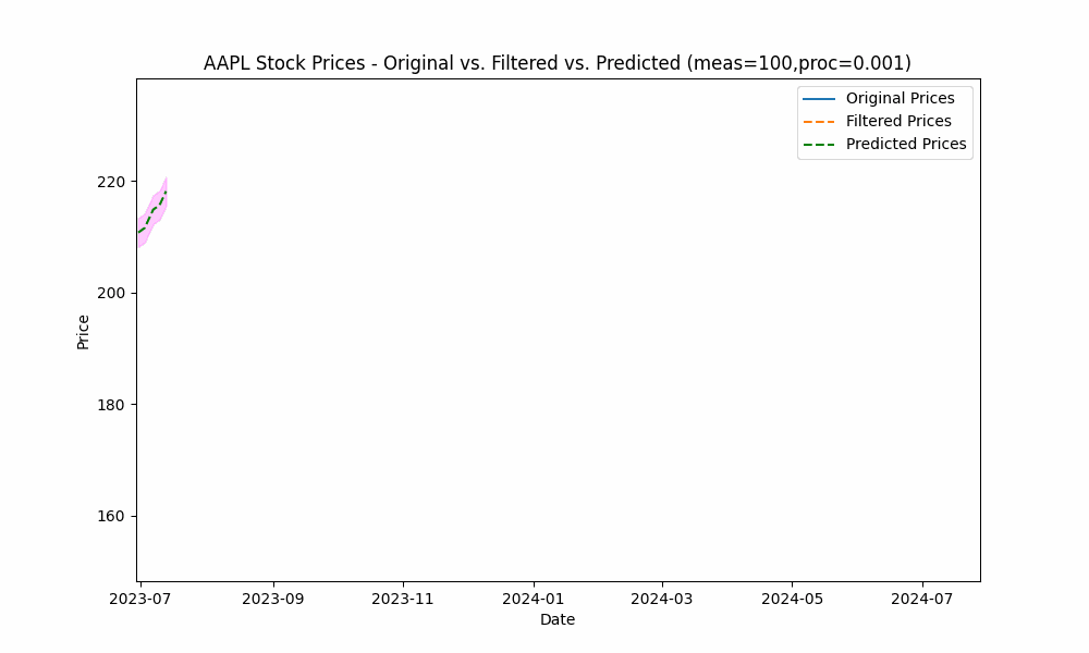
By focusing even more on the process model (e.g. setting the measurement noise scale to 100 and process noise scale to 0.001), we see the filter has the smoothest filtering yet.
In the next plot, we overlay the band created by projecting the previous rolling 20 period standard deviation onto the future predictions to see how well the actual prices fit within our prediction band.
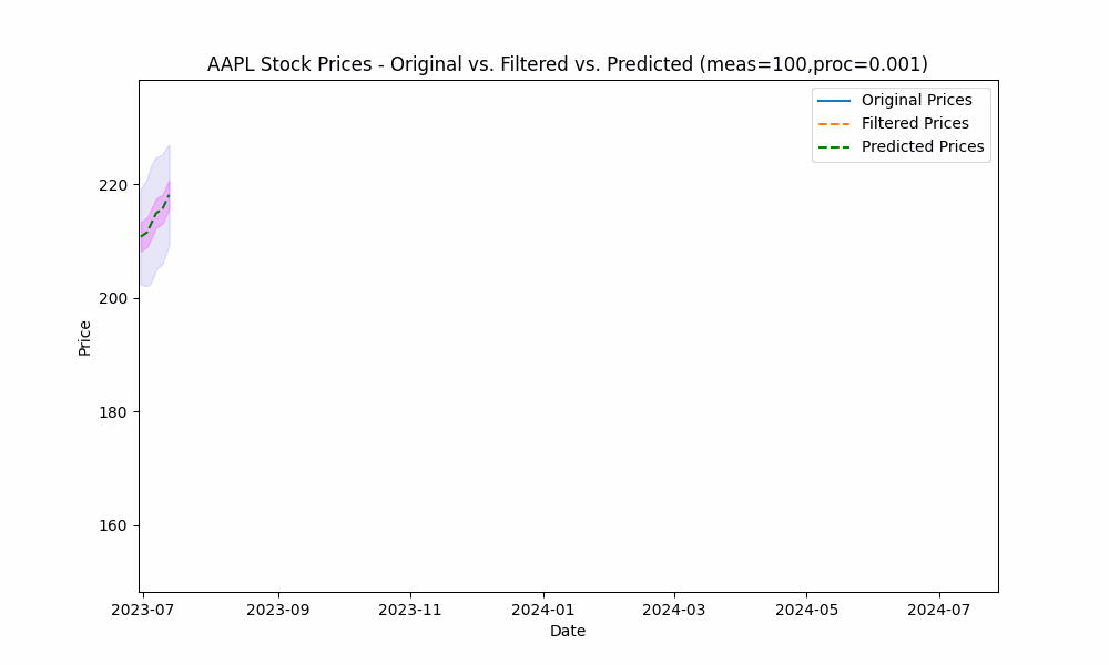
From the animation above we see that the price fits within the prediction band well except when rapid, sustained price changes occur.
By using the less smoothed filter with a Measurement Noise Scale = 10, we capture most of the price volatility within the single standard deviation band.
Summary

In this post we discussed the Kalman Filter and Unscented Kalman Filter including how these filters are used. More specifically we discussed how to initialize the Unscented Kalman Filter (UKF) to filter stock prices and demonstrated this filtering with several different smoothing settings. Using the Kalman Filter and Unscented Kalman Filter have been shown to generate excess returns in pair-based trading strategies [7] and in portfolio selection strategies [8].
To see the full Python code used in this pose, see the Kalman Filter Example on GitHub.
Happy deep learning with the Unscented Kalman Filter!
[1] A New Approach to Linear Filtering and Prediction Problems, by R. E. Kalman, 1960, ASME
[2] KalmanFilter.NET, by Alex Becker, 2024
[3] Kalman-and-Bayesian-Filters-in-Python, by Roger Labbe, 2022, GitHub:rlabbe
[4] The Unscented Kalman Filter for Nonlinear Estimation, by Eric A. Wan and Rudolph van der Merwe, 2004
[5] GitHub: filterpy, by Roger Labbe, 2015, GitHub
[6] Sigma-Point Kalman Filters for Probabilistic Inference in Dynamic State-Space Models, by Rudolph van der Merwe and Eric A. Wan, 2004
[7] Research on Hierarchical Pair Trading Strategy Based on Machine Learning and Kalman Filter, by Shuo Yang, Ke Huang and Yao-wen Chen, 2023
[8] Kalman Filtering and Online Learning Algorithms for Portfolio Selection, by Raphael Nkomo and Alain Kabundi, 2013, ERSA